Localised rare-earth and actinide ions are well described by ![]() -coupling with a ground state multiplet determined by Hund's Rules, and characterised by the total angular momentum quantum number
-coupling with a ground state multiplet determined by Hund's Rules, and characterised by the total angular momentum quantum number ![]() . In a free ion, these
. In a free ion, these ![]() -multiplets containing
-multiplets containing ![]() levels labeled by
levels labeled by
![]() are degenerate. However, crystal field interactions arising from the breaking of the symmetry of free ions by the regular arrangements of a crystal will break this degeneracy of the free ion
are degenerate. However, crystal field interactions arising from the breaking of the symmetry of free ions by the regular arrangements of a crystal will break this degeneracy of the free ion ![]() multiplets. This occurs because whereas a free ion will have a Hamiltonian with spherical symmetry, the magnetic ions in a crystal will have a different site symmetry.
multiplets. This occurs because whereas a free ion will have a Hamiltonian with spherical symmetry, the magnetic ions in a crystal will have a different site symmetry.
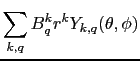
Thus the effect of a crystal field can be thought of as a perturbation acting on free magnetic ions due to the mechanisms of crystal bonding. Initially it was attributed to the electric potential due to the charge distribution of surrounding ions on a magnetic ion within the crystal, hence the term crystalline electric field. Expressing this contribution by a multipolar expansion centred on the magnetic ion yields the crystal field potential as a sum over spherical harmonics ![]()
![]() are crystal field parameters which determines the strength the interaction. The order
are crystal field parameters which determines the strength the interaction. The order ![]() runs over even integers up to
runs over even integers up to ![]() where
where ![]() is the orbital angular momentum number of the equivalent electrons in question. Thus for rare earth ions, it is 3, and
is the orbital angular momentum number of the equivalent electrons in question. Thus for rare earth ions, it is 3, and ![]() . The component
. The component ![]() runs over
runs over
![]() .
.
In order to calculate the Hamilton matrix for the crystal field interaction we have to express the CF potential as an operator
![]() whose matrix elements may be easily calculated. Then the eigenvalue problem
whose matrix elements may be easily calculated. Then the eigenvalue problem
![]() may be solved to find the energies
may be solved to find the energies ![]() (to an arbitrary constant shift) and wavefunctions
(to an arbitrary constant shift) and wavefunctions
![]() of the magnetic ion in the crystal field. We now come to a problem of notation and normalisation. The first formalism to handle crystal fields was developed by Stevens using operator equivalents [Stevens(1952)]. Stevens first expressed the term
of the magnetic ion in the crystal field. We now come to a problem of notation and normalisation. The first formalism to handle crystal fields was developed by Stevens using operator equivalents [Stevens(1952)]. Stevens first expressed the term
![]() in Cartesian coordinates, to obtain for example,
in Cartesian coordinates, to obtain for example,
![]() , where we have ignored a constant term in the spherical harmonics. He then used the result that within a manifold of constant
, where we have ignored a constant term in the spherical harmonics. He then used the result that within a manifold of constant ![]() - such as the ground
- such as the ground ![]() state of a rare earth ion - the potential operator
state of a rare earth ion - the potential operator
![]() is equivalent to a similar angular momentum operator formed by taking the Cartesian expression of the potential operator, replacing terms in
is equivalent to a similar angular momentum operator formed by taking the Cartesian expression of the potential operator, replacing terms in ![]() by terms in
by terms in
![]() and symmetrising to allow for the non-commutation of
and symmetrising to allow for the non-commutation of
![]() . The two expressions are then related by an operator equivalent factor,
. The two expressions are then related by an operator equivalent factor,
![]() for
for ![]() respectively. Thus, for the
respectively. Thus, for the ![]() terms, for example we have:
terms, for example we have:
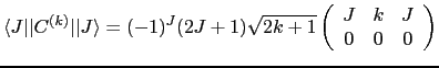
Stevens then listed the matrix elements for these three operators, and later he and others added matrix elements of all terms with even ![]() [Jones et al.(1959)Jones, Baker, and
Pope], which enables magnetic ions in sites of orthorhombic (
[Jones et al.(1959)Jones, Baker, and
Pope], which enables magnetic ions in sites of orthorhombic (![]() space group) or higher symmetry to be calculated. The expressions in the angular momentum operators given in equations 2 are termed Steven's operators
space group) or higher symmetry to be calculated. The expressions in the angular momentum operators given in equations 2 are termed Steven's operators ![]() by later authors, and are listed for all
by later authors, and are listed for all ![]() and
and
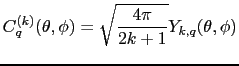
![]() by Smith and Thornley [Smith and Thornley(1966)]. The CF parameters are now specified by
by Smith and Thornley [Smith and Thornley(1966)]. The CF parameters are now specified by ![]() , so that the crystal field operator is:
, so that the crystal field operator is:
where the operator equivalent factors ![]() is
is
![]() respectively for
respectively for ![]() , after the notation of Judd. These factors were listed for the ground states of the rare earths by Stevens, and a method to calculate the values for other
, after the notation of Judd. These factors were listed for the ground states of the rare earths by Stevens, and a method to calculate the values for other ![]() states was given by Elliot et al. [Elliot et al.(1957)Elliot, Judd, and
Runciman]. Although both
states was given by Elliot et al. [Elliot et al.(1957)Elliot, Judd, and
Runciman]. Although both ![]() and
and
![]() may be calculated separately from models, we choose to regard both as a single parameter to be varied, and henceforth will refer to
may be calculated separately from models, we choose to regard both as a single parameter to be varied, and henceforth will refer to
![]() as crystal field parameters under Steven's normalisation. This is because the main use of the SAFiCF program is to fit crystal field parameters to an phenomenological model rather than to compare with theoretical models of the crystal field.
as crystal field parameters under Steven's normalisation. This is because the main use of the SAFiCF program is to fit crystal field parameters to an phenomenological model rather than to compare with theoretical models of the crystal field.
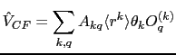
However Steven's methods, whilst effective for hand calculations is not efficient for machine calculations as it would require inputing tables of matrix elements (which may be prone to error, and be hard to debug) and looking up their values. Instead we shall follow the later methods of Wybourne, Judd and others, using the tensor operator techniques due first to Racah [Judd(1998)]. We express the crystal field potential operator in terms of a tensor operator ![]() which transforms in the same way as the quantities:
which transforms in the same way as the quantities:
This defines the normalisation of the crystal field parameters, and is called the Wybourne normalisation by Newman and Ng [Newman and Ng(2000)] 1. The crystal field operator is now expressed as:
such that
![]() is hermitian and the parameters
is hermitian and the parameters ![]() are real. The matrix elements of
are real. The matrix elements of ![]() may be calculated first by factorising into a part dependent only on
may be calculated first by factorising into a part dependent only on ![]() and
and ![]() , and reduced matrix element dependent on
, and reduced matrix element dependent on ![]() and
and ![]() by application of the Wigner-Eckart theorem:
by application of the Wigner-Eckart theorem:
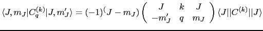
The reduced matrix element
![]() is just a number and is given by:
is just a number and is given by:
where the large brackets denotes a Wigner ![]() symbol, which is related to the Clebsch-Gordan coefficients resulting from the coupling of two angular momenta.
symbol, which is related to the Clebsch-Gordan coefficients resulting from the coupling of two angular momenta.
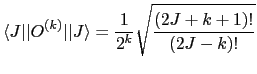
However, because the Steven's normalisation is still widely in use, SAFiCF defaults to using it, rather than the Wybourne normalisation. In this case, whilst the ![]() and
and ![]() dependent parts of the matrix elements are the same, we need to replace the reduced matrix element
dependent parts of the matrix elements are the same, we need to replace the reduced matrix element
![]() by another reduced matrix element appropriate to the Steven's operators [Smith and Thornley(1966)]:
by another reduced matrix element appropriate to the Steven's operators [Smith and Thornley(1966)]:
This result may be derived by first taking the ![]() components, and constructing the diagonal matrix elements for the operators in equations 2. The Wigner-Eckart theorem then gives:
components, and constructing the diagonal matrix elements for the operators in equations 2. The Wigner-Eckart theorem then gives:
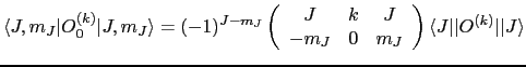
Taking ![]() , we find that
, we find that
![]() , and using the algebraic expression for the 3
, and using the algebraic expression for the 3![]() symbol in the above equation2:
symbol in the above equation2:
![$\displaystyle \left( \begin{array}{ccc} J & 2 & J -m_J & 0 & m_J \end{array} \right) = (-1)^{J-m_J} \frac{2(3m_J^2 - J(J+1)}{[(2J+3)!/(2J-2)!]^\frac{1}{2}} $](img57.png)
we arrive the result 8 with ![]() . Similar techniques for
. Similar techniques for ![]() and
and ![]() yields the
yields the ![]() terms in equations 8.
terms in equations 8.
These equations to calculate the crystal field Hamilton matrix within a constant ![]() -manifold is implemented in the function cf_hmltn(J,A2,A4,A6), which by default assumes that the CF parameters, expressed as
-manifold is implemented in the function cf_hmltn(J,A2,A4,A6), which by default assumes that the CF parameters, expressed as ![]() component vectors A2,A4,A6, are in Steven's normalisation3.
component vectors A2,A4,A6, are in Steven's normalisation3.
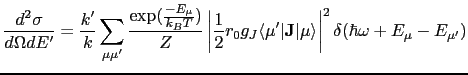
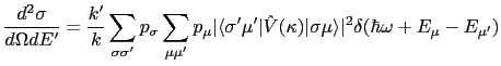
We now turn to the interaction of the neutron with the electrons of the magnetic ions in a crystal field. Approximating the neutron wavefunction as a plane wave and using Fermi's Golden Rule to obtain the transition probability, then multiplying this by the density of neutron final states and dividing by incident neutron flux (which quantities are proportional to ![]() ), the double differential cross-section is:
), the double differential cross-section is:
where ![]() and
and ![]() are the wavevectors of the initial,
are the wavevectors of the initial, ![]() , and final,
, and final, ![]() , states of the target ion. The neutron's initial and final polarisation is labeled by
, states of the target ion. The neutron's initial and final polarisation is labeled by ![]() and
and ![]() respectively, and
respectively, and ![]() is the initial probability distribution of the neutron's spin, whilst
is the initial probability distribution of the neutron's spin, whilst ![]() is the probability distribution of initial target states.
is the probability distribution of initial target states.
![]() is the wavevector transfer, and
is the wavevector transfer, and
![]() is the neutron-atom interaction operator.
is the neutron-atom interaction operator.
For magnetic scattering only (ignoring neutron-nuclear interactions), the neutron-electron interaction operator is:
Where
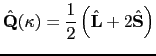
![]() is the intermediate scattering operator, which is the Fourier transform of the magnetisation density, and has spin and (orbital) momentum dependent parts. In the limit
is the intermediate scattering operator, which is the Fourier transform of the magnetisation density, and has spin and (orbital) momentum dependent parts. In the limit
![]() , however, we can use the dipole approximation, and obtain:
, however, we can use the dipole approximation, and obtain:
SAFiCF does not handle polarised neutrons at present, but we hope to implement it in a future version, so for now, we will omit the sums over ![]() . Furthermore, we take the ideal case where
. Furthermore, we take the ideal case where
![]() , and for Russel-Saunders (
, and for Russel-Saunders (![]() ) coupling replace
) coupling replace
![]() by
by
![]() obtain:
obtain:
Where
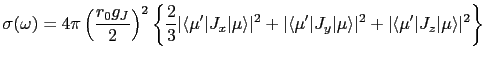
![]() is the partition function. We can now average over solid angle to obtain the cross-section at the energies of the transitions between electronic states
is the partition function. We can now average over solid angle to obtain the cross-section at the energies of the transitions between electronic states
![]() :
:
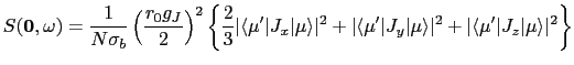
Alternatively, we can calculate the scattering function at ![]() :
:
where ![]() is the number of scatterers and
is the number of scatterers and ![]() is their scattering length. The two equations 12 and 13 are calculated by the function cflvls(Hcf,T) where Hcf is the crystal field Hamilton matrix calculated as described above by cf_hmltn. The matrix elements
is their scattering length. The two equations 12 and 13 are calculated by the function cflvls(Hcf,T) where Hcf is the crystal field Hamilton matrix calculated as described above by cf_hmltn. The matrix elements
![]() are calculated from the matrix elements of
are calculated from the matrix elements of ![]() as described above also, by
as described above also, by
![]() ,
,
![]() and
and
![]() by the function mag_op_J(J).
by the function mag_op_J(J).
Finally, we note that this treatment of inelastic neutron scattering by magnetic ions in a crystal field is an approximation which may not agree with measurements. In particular, the magnetic form factor for real measurements with
![]() will change the intensity of spectra, and the neutron-electron operator will no longer be proportional to
will change the intensity of spectra, and the neutron-electron operator will no longer be proportional to
![]() . A more sophisticated technique is described by Balcar and Lovesey [Balcar and Lovesey(1989)], again using Racah tensor operator techniques, and will be implemented in future versions which will also include calculations of the crystal field levels of ions in intermediate coupling.
. A more sophisticated technique is described by Balcar and Lovesey [Balcar and Lovesey(1989)], again using Racah tensor operator techniques, and will be implemented in future versions which will also include calculations of the crystal field levels of ions in intermediate coupling.
![$\displaystyle \hat{V}_{CF} = \sum_{k,q<0} i B_q^k \left[ C_{\vert q\vert}^{k} -...
...B_0^k O_0^{(k)} + \sum_{k,q>0} B_q^k \left[ C_q^{k} + (-1)^q C_{-q}^{k} \right]$](img46.png)
![$\displaystyle \hat{V}_M(\mathbf{\kappa}) = r_0 \hat{\mathbf{\sigma}} \cdot \fra...
...appa^2} [ \mathbf{\kappa} \times \{\hat{\mathbf{Q}} \times \mathbf{\kappa} \} ]$](img72.png)